Disclaimer: I am not a financial expert. I am a student in statistics and probability. What follows is some exposition on an exercise found in one of my textbooks. It was not a trading book, but rather a book on actuarial models for insurance. I thought it was interesting, and decided to write about it.
I.
On finance.yahoo.com, stock price data can be easily downloaded and analyzed. Here, we consider a stock and a cryptocurrency, Google and Bitcoin, which are words that have passed through the lips of pretty much every person who knows what an investment is. Bitcoin, in particular, was the source of many a meme, when the lovable cryptocurrency topped out in value at $19345.49. Google, on the other hand, is an actual company, with investors and products, and likely was what you used in order to find this blog. Now, if you had some fixed  amount of money, where should you invest it? Can we make a decision based only on historical data and some very elementary risk measures? (NB: No, we cannot. If such elementary machinery provided any substantial predictive power for return on investment, then nearly anyone comprehending basic calculus and probability theory would be wildly rich. However, this makes an interesting exercise.)
II.
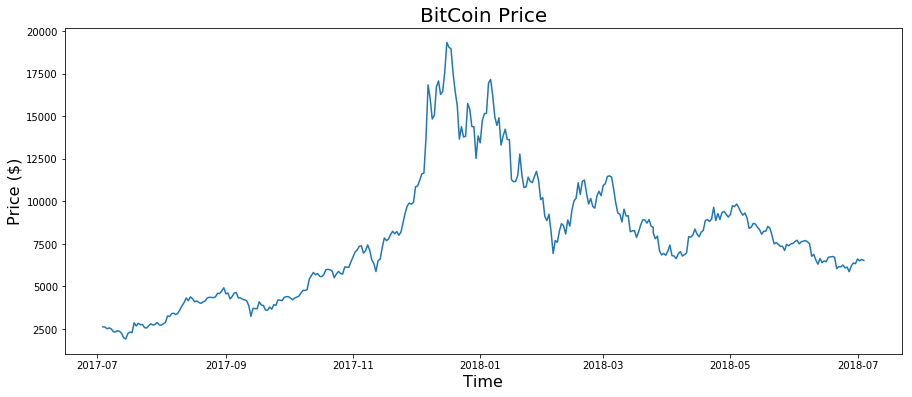
From finance.yahoo, we consider historical stock price data from 2017-05-05 to 2018-05-05 (essentially present day, at the time of this writing). In this case, we will look at the Close price. Here is the time series of the Bitcoin closing price (366 observations):
And we also have the Google price data (255 observations – some days are missing in the data because of holidays, or an error on the part of finance.yahoo. Ideally, we would want to have data with the same number of observations, but since this isn’t a “serious” exercise, we can say that this is good enough).

We can see that clearly both Bitcoin and Google saw big increases in price around the start of 2018, but the closing prices for bitcoin appear to be dropping as 2018 continues on, yet Google has remained relatively high. Because stock prices are effectively stochastic, ie, random, we really cannot draw any conclusions based on these charts alone. Though, some speculate that bitcoin prices are going to take off again at some point (“To the moon!”). If all I knew were these charts, it would be difficult to discern which asset will make you more money. Though, perhaps I would be tempted to go bitcoin, as its apparently high volatility may indicate another large spike in price in the future. In fact, what can we say about the returns of these two assets?
A return is defined as the formula every business major knows:  . We will use a modified version of this formula that is simply a ratio of the price from yesterday and the price today. That is, we will define a daily return
  as the ratio
 .
.
So it follows that when  , we saw a gain, and when $ latex V < 1$, we saw a loss. If
  , then naturally we didn’t lose or gain anything. However, here is essentially a continuous random variable, so the probability that exactly is 0. We can thus expect to either gain or lose money when considering the returns in a 24 hour period. While we could extend our time interval to beyond 24 hours, we consider only the returns on a single day – we are pretending to be day traders here.
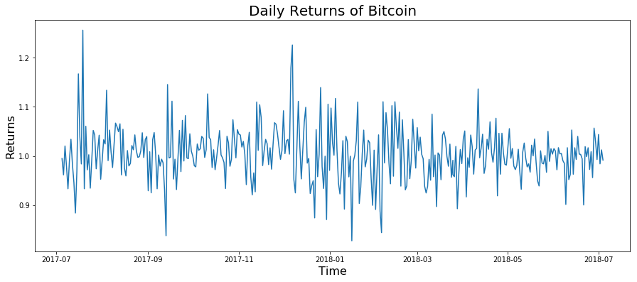

The graphs of the daily returns from both assets appear to resemble white noise, which is indicative that the returns are approximately normally distributed. (A lie. Keep going). This is actually a key assumption in proceeding with our analysis, so it is pertinent to take a glance at the quantile-quantile plots as well:
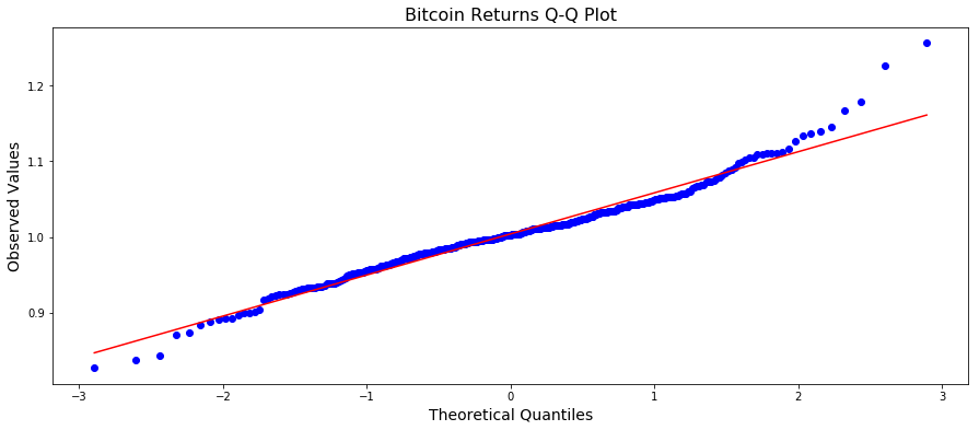
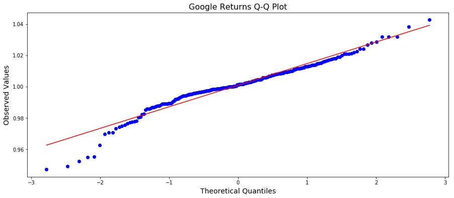
Both data sets are probably close enough. There is a bit of fuzziness in the tails here, and some skewness (in particular, Google has some right tail skew), but it’s not totally unreasonable to assume that the data are approximately normally distributed.
(NB: We are fibbing a bit. Because the definition of returns we are using is simply a ratio, they are actually not normally distributed, as the return is strictly greater than zero. In The Black Swan, Nassim Nicholas Taleb argues heavily against the profilic use of assuming the normal distribution in the financial sector – and for good reason. Bad assumptions on models can be disasterous and it’s a generally unwaranted assumption, for actual return data has fatter tails than a normal distribution. However, since it is better to beg for forgiveness rather than permission, we will take our returns data as approximately normal, and continue with the exercise. Our aim here is to explore the concept of risk and utility; not to argue about the distribution of returns.)
It’s a relatively common assumption to assume that the daily returns are a stochastic variable, and so we can let  denote the random return for the Bitcoin asset and
  denote the return of the google asset. Using the data we have on the daily returns, we can estimate the mean
  and standard deviation
  using the arithmetic mean and sample standard deviation. We have:


On inspection, it appears that the Bitcoin asset gives a higher average return than the Google asset, however, it suffers from a higher standard deviation, which is indicative of more volatility – you are more likely to get larger spikes of gains, as well as larger spikes of losses. Perhaps this is to be expected.
III.
(NB: The following conversation may be skipped for those who are well acquainted with VaR and its concepts.)
The Value-at-Risk (VaR) criterion is, as defined in Rotar’s Actuarial Models: The Mathematics of Insurance is the “smallest value  for which
  . Or, more formally, we can write, for a random variable
 .
.
This is a definition of the  -quantile of a random variable .
This can also be said to be the value at  level of risk. For example, if we set
  , and is a random variable denoting income, then
  is the smallest income we can expect to occur among all possible income values with probability 95%. That is, the probability we have an income smaller than
  occurs with only probability 5%. This is how we can use a notion of “risk” in finance. We are, in essence, trying to calculate how much money we stand to lose at certain probabilities. There are several ways of doing this. We can either place the VaR criterion on a distribution of losses, or we can place the VaR criterion on a distribution of income, and thereby calculate our losses as a function of our income at some level of risk. For example, if we bet $10,000 on a particular asset, and we calculate the VaR for income, we can see what our losses will be as a function of our bet. If the value at 5% risk (on our income) ends up being $7000 dollars, then that means 5% of the time, we stand to lose $3000. (This does not seem like a very good bet).
We can also place this VaR on a distribution of losses, where the random variable  takes on negative values. In this case, we get our losses instantly. In our example, the value at risk at 5% is -$3000 dollars. By calculating our “risk” in this manner, we can obtain information about what is at stake in our financial bets.
Since we can choose , we can essentially estimate our income at whatever level of risk we want. In this definition, if  is negative, than this corresponds to losses.
We say that we prefer over  when
when  , and in this case we write
  .
.
Now for the relevant part. From Actuarial Models: Suppose we have a normally distributed random variable with mean and standard deviation . Now if  is the distribution function of , the -quantile of is a solution to the equation
  . If we denote
  the -quantile of the standard normal distribution, so that
  , then we can rewrite the equation as
  . Thus, we get:
 .
.
Since multiplying a normally distributed random variable by a constant results in a normally distributed random variable, this means we can actually compute the value at risk in our investments in Bitcoin and Google assets, as the daily returns are (approximately) normally distributed. If we think of the amount of money we invested as a weight or scalar (say n dollars), we can define a new random variable  that denotes our expected income from our investment. Then, the expected value of
  is
is ![E[X^*] = nE[X] = n\mu](https://s0.wp.com/latex.php?latex=E%5BX%5E%2A%5D+%3D+nE%5BX%5D+%3D+n%5Cmu%C2%A0&bg=ffffff&fg=000000&s=1&c=20201002) and the standard deviation is
and the standard deviation is  . Thus, we get for the VaR criterion,

Since we are generally interested in small probabilities (as we are primarily interested in this notion of risk), we will take  , which implies that
  . Essentially, we want the expected return on investment to be as high as possible, while the standard deviation can be seen as a measure of riskiness. Since we are looking at small probabilities and assuming a normal distribution, the quantile
  will always be negative, and so the higher the standard deviation, the higher the level of riskiness (as we are in a position to actually lose money if the prices drop too much unexpected).
IV.
By the preceding discussion, we can suppose that we are willing to invest n dollars into either Bitcoin or Google. We will assume that the better choice of investment will be the asset that has a smaller risk. Under the VaR criterion, we want to see which asset will not only make us the most money, but has the smallest penalty should something bad happen – like an unexpected drop in prices. Since this is based on our definition of return as a ratio, the absolutely value in the price shouldn’t matter from a mathematical point of view.
Define  as the expected income from the Bitcoin investment and define
  as the expected income from the Google investment. We will fix n for now. Also set
  . Now, we have, by our estimates via the price datasets,
![q_\gamma(X^*) = nE[X] + n q_{\gamma s}SD(X) = n(1.0040) - n1.96(0.0547)](https://s0.wp.com/latex.php?latex=q_%5Cgamma%28X%5E%2A%29+%3D+nE%5BX%5D+%2B+n+q_%7B%5Cgamma+s%7DSD%28X%29+%3D+n%281.0040%29+-+n1.96%280.0547%29+&bg=ffffff&fg=000000&s=1&c=20201002) (1)
(1)
![q_\gamma(Y^*) = nE[Y] + n q_{\gamma s}SD(Y) = n(1.0009) - n1.96(0.0140)](https://s0.wp.com/latex.php?latex=q_%5Cgamma%28Y%5E%2A%29+%3D+nE%5BY%5D+%2B+n+q_%7B%5Cgamma+s%7DSD%28Y%29+%3D+n%281.0009%29+-+n1.96%280.0140%29+&bg=ffffff&fg=000000&s=1&c=20201002) (2)
(2)
We now have a function of our investment n which we can plot in Python:
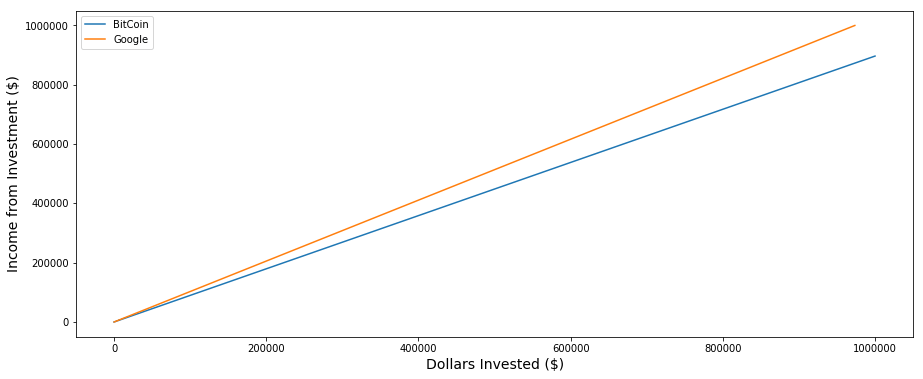
We can see that the more money we invest at a time, the larger the VaR for the Google asset. As a concrete example, if we compare an investment of $10,000 in Google and Bitcoin, then our value at 2.5% risk for both assets is


By definition of VaR, this means that 2.5% of the time, we stand to lose $1,032.12 dollars on Bitcoin, but only $265.4 dollars on Google. Bitcoin is a riskier bet. This is intuitively obvious just from looking at the larger standard deviation. The investor is in a position to lose (or gain) much more money than in a bet with a higher variance. Based on this analysis, it seems that the choice of investment should be in the Google asset. Since denotes the income from Bitcoin and denotes the income from Google, and we have that the value-at-risk is higher for Google, we would say that we prefer Google, and write the equation  .
.
But is this result generalizable to all humans? Should every investor make this choice? Perhaps, but we know that human beings are not always rational, but nevertheless their behavior can sometimes be modeled as maximizing some kind of utility function. I don’t know what my utility function is, but for whatever reason, the utility out of typing up this blog post is higher than the utility I get from doing homework.
V.
Utility functions are, in essence, some way of characterizing human behavior. Human beings all want something, and that something is often fairly intangible. Yet, one utility that seems “modelable” is the utility of money. Money gives us utility almost however you define it, since money can serve as a proxy for the things we actually want — be it power, sex, or even a new video game. (I may not value money at all as an axiom, but if I value playing video games, then I value free time so that I can play video games, and also the money required to purchase them. Ergo, I have a job that gives me weekends off. This property of valuation seems to hold almost everywhere in adults that like video games, except on the set of video-game pirating NEETs, e.g., 4channers, which is a set of small measure.)
If we take it as an axiom that every human has some innate, unknown utility function, and that human beings are, in general, utility maximizers, then we can use some relatively simple mathematics to model a person’s behavior. There are caveats. One can never assume that a model is true, as true behavior (of anything) is inherently unknowable (empiricism helps, but only serves to make models more accurate. Not more true).
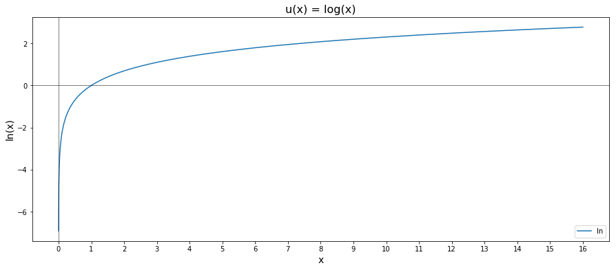
Here we denote a utility function by u. A classical example of a utility function is the natural logarithm  , where
  is some number representing capital.
The expected utility maximization criterion is an axiom that if someone is a utility maximizer, then they would prefer an investment strategy over if and only if the expected utility payoff of is higher than the expected utility pay off of . That is
![X \succeq Y \iff E[u(X)] \geq E[u(Y)]](https://s0.wp.com/latex.php?latex=X+%5Csucceq+Y+%5Ciff+E%5Bu%28X%29%5D+%5Cgeq+E%5Bu%28Y%29%5D%C2%A0&bg=ffffff&fg=000000&s=1&c=20201002) .
.
Perhaps the simplest utility function is simply dollar amounts, but it doesn’t capture the inherent decision making process used by actual humans. How people characterize their investments has a lot to do with how the feel about them, and their expected return, and the potential risks involved in some strategy. That’s where a utility function comes in — it is an attempt to capture some of those decision making processes.
We will avoid some details here, but essentially investors (or gamblers) can be described as either being risk averse, risk taking, or risk neutral. An investor who is risk averse is an investor who, naturally, prefers stability from their assets. Since the VaR for the Google asset is higher than the VaR for Bitcoin, a risk averse investor would be more inclined to invest in Google over Bitcoin. However, Bitcoin, has a larger variance, and so there is a probability of a large spike in price – and that means someone is potentially makes a lot of money. An investor who still prefers Bitcoin despite the lower VaR could be said to be a risk-taker. He or she is willing to invest the money and take the risk of losing it for the (likely small) probability of a large pay off.
Utility functions don’t have to be positive (note that the natural log is not strictly postive). And since we only care about maximizing our “utils”, we can actually use the natural logarithm to model investment strategy behavior in a “rational” human being. As  , we have that
  . This says that an investor is absolutely interested in getting more capital, as that will give him greater utility. But after amassing a large enough amount of capital, the function slows down considerably. This makes sense: once you have $1,000,000 how much more utility do you get out of a couple more bucks? Once you’re Bill Gates, how much more utility do you get out of any amount of money? (Technically, since the natural logarithmic function is unbounded, there is some amount of money Bill Gates would eventually want to acquire. This perhaps does not reflect reality, in that Bill Gates has so much money that it’s pretty much incomprehensible. I cannot imagine what it must be like to be so rich that you couldn’t spend it all — even if you tried).
But on the other hand, since the natural logarithm diverges to  as our capital decreases to zero, we are essentially “very afraid” of being ruined. We want as much money (utility) as possible, but not so badly that we are willing to go completely broke. (This function ignores the key fact that many Americans are actually in debt, negative capital, but that is perhaps a post for another time). This seems to provide a reasonable utility function for actual human behavior. Again, this function is not underlying truth, but rather an attempt to model something. Models are incorrect, since they are estimators, but can be made more accurate.
Passing the return data from both Bitcoin and Google and taking a mean gives an expected “utility” of 0.0025 for Bitcoin and 0.0008 for Google – in this scenario, we actually prefer to invest in Bitcoin.
(This procedure may seem ad-hoc, but has some justification. Let  be random variables denoting the 1 day returns for n days. The Expected Utility Maximization criterion (EUM) is defined so that we care about the expected utility of an investment plan. If denotes the (day-trading) investment plan pertaining to returns
  , then we can estimate the expected utility by passing the n returns through a utility function u and taking the mean. By the law of large numbers, this will be approximate to the true expected value. That is,
![\frac{u(X_1) + u(X_2) + ... + u(X_n)}{n} \approx E[u(X)]](https://s0.wp.com/latex.php?latex=%5Cfrac%7Bu%28X_1%29+%2B+u%28X_2%29+%2B+...+%2B+u%28X_n%29%7D%7Bn%7D+%5Capprox+E%5Bu%28X%29%5D%C2%A0&bg=ffffff&fg=000000&s=1&c=20201002)
by the law of large numbers when n is large. )
What about a different utility function? Consider the utility function  . This is called a quadratic utility function, and is actually a function of the mean and variance, and so, heuristically, it may be a more “objective” criterion in terms of asset assessment, as we really only care about our expected returns and our possibility of a loss. For a simple proof that this quadratic function really is a function of the mean and variance, recall that
 ![Var(X) = E[X^2] - E[X]^2](https://s0.wp.com/latex.php?latex=Var%28X%29+%3D+E%5BX%5E2%5D+-+E%5BX%5D%5E2+&bg=ffffff&fg=000000&s=1&c=20201002) . Therefore,
. Therefore, ![E[X^2] = Var(X) + E[X]^2](https://s0.wp.com/latex.php?latex=E%5BX%5E2%5D+%3D+Var%28X%29+%2B+E%5BX%5D%5E2%C2%A0&bg=ffffff&fg=000000&s=1&c=20201002)
![E[u(X)] = E[2aX - X^2] = 2aE[X] - E[X^2] = 2aE[X] -(Var(X) + E[X]^2)](https://s0.wp.com/latex.php?latex=E%5Bu%28X%29%5D+%3D+E%5B2aX+-+X%5E2%5D+%3D+2aE%5BX%5D+-+E%5BX%5E2%5D+%3D+2aE%5BX%5D+-%28Var%28X%29+%2B+E%5BX%5D%5E2%29&bg=ffffff&fg=000000&s=0&c=20201002)
And this simply becomes  , which completes the proof. Now, for the scalar a; one of the requirements for a utility function is that the function is non-decreasing. We can strengthen this slightly to make it an increasing function, (so that more capital or a higher return means that we get a higher utility, matching our intuition), and so we need to pick a so that
  for every choice of x. In other words, we want
  . Our returns for both data sets are not higher than 1.25, so we can pick
  , so that our utility function is then
  . Like before, we can estimate the expected utility from our strategies by passing the returns through this utility function and taking the mean. So, recalling that is our Bitcoin strategy and
  is our Google strategy,
![E[u(X)] \approx 1.4989](https://s0.wp.com/latex.php?latex=E%5Bu%28X%29%5D+%5Capprox%C2%A01.4989+&bg=ffffff&fg=000000&s=1&c=20201002)
![E[u(Y)] \approx 1.5003](https://s0.wp.com/latex.php?latex=E%5Bu%28Y%29%5D+%5Capprox+1.5003+&bg=ffffff&fg=000000&s=1&c=20201002)
So our expected utility is now slightly higher for the Google strategy, which matches our intuition from the VaR criterion. (However, the difference between the two is extremely small, and increasing a results in us preferring Bitcoin again. Utility seems to be quite finicky).
VI.
So, which is it? Google or Bitcoin. I’m sorry to have to give a non-answer, but the non-answer is that it depends on your utility function. If you decide that the VaR criterion is “good enough” to decide on which to invest in, then perhaps you’re very risk averse, your utility function is concave. In that case, Google seems like a safe bet. Even safer – a mutual fund. If, however, you’re willing to shoulder the risk of losing everything at the prospect of big gains, then obviously bitcoin is the answer here, as it has been for many other individuals. However, modeling risk seems like a general good idea. It’s why traders seem to espouse having diversified portfolios (there is a very simple mathematical proof for why this reduces variance, and thus risk, of your investments. But even heuristic reasoning may suffice. If all your eggs are in one basket, and that basket gets hit with a financial nuclear bomb, then you lose all your eggs. If you have many baskets, and one egg in each, then losing one basket means you only lost one egg — that is, one investment.)
****
Caveats and further questions:
i) As expressed earlier, the distribution of returns is mostly not normal. It is a very strong and simplifying assumption, which is why it is done, but by assuming the distribution of returns is normal, and then calculating the VaR at a particular percentage analytically, the actual chance of the risky event occurring is higher – perhaps much higher. There are non-parametric methods that exist, which make no assumptions about a distribution and work entirely on historical data. This is called historical simulation. There is another method that uses Monte Carlo methods, but I don’t know much about that, yet. These methods are likely more robust, in that they use less assumptions.
ii) Utility functions as a means to optimize a portfolio seem weird to me. A utility function is a function that essentially describes the behavior of an individual by attaching “utils” to some notion of having more or less of something. This criteria for portfolio optimization is used, indeed, but I don’t know enough about it to really comment deeply. Maybe another time.
iii) There is a critical error of VaR in which Taleb occasionally critiques. When you fix a probability level, say 1%, and then calculate VaR, you make the very explicit assumption that events with probability less than 1% do not occur. This is perhaps certifiable madness in finance. If you take the stock market as entirely stochastic, which many people do thanks to the Efficient Market Hypothesis, then the stock price movements are a random walk. Since a random walk does not depend on the past at all, and markets are here to stay, eventually a “rare event”, one that occurs with probably less than 1% is bound to happen, for someone, somewhere. And here’s the problem – value at risk assumes that it doesn’t. This may not be a big deal, but there isnt’ evidence that risk and expected losses at a particular risk level are linear. In fact, as Taleb argues, it is these rare events, these Black Swans that are most impactful, most disastrous. It’s possible that while you can manage the loss of a 1% event, a 0.5% event could liquidate your company. That said, all is not lost for VaR. Part of managing risk is having a “risk measure”, in which multiple risk criterion are considered and given relative weights dependent on the concerns of the individual or the firm. There is, also, Conditional VaR, or “expected shortfall” which tries to estimate the impact of extremely rare events. Moreover, there are many other risk criterion than those two, enough to fill a textbook on the subject.
iv) I am not a trader, but I am curious about a trading strategy for the individual: I believe that one could come up with a coherent risk measure that appeals to them, and simply evaluate many stocks on that risk measure, and then pick the stocks based on obtaining the smallest amount of risk, with some ratio of highest expected returns. This is a thing for portfolio management in the investment industry in which there are ample resources (google “risk parity”), but I wonder if it could be specified into a coherent strategy for the individual with regular-person level resources. I am likely missing something here, as this seems obvious to me, but I am not a trader and thus have not read any trading books. It’s possible that this is a strategy considered in chapter 1 of some book somewhere, but I also get the feeling that this method would be too computationally intensive for the general public, but would appeal to the analytically minded. If anyone knows, let me know. I might try and explore this idea.
v) The data at the time of this writing is already outdated. I figure that is probably just okay.
vi) Future project: investigate the Efficient Market Hypothesis by trying some machine learning techniques on stock data. Does the past model the future? Economists say no, but economists also failed to predict the 2008 crash, and the Efficient Market Hypothesis precludes the idea of a bubble and the event of a crash, so definitely worth looking into. In fact, Bitcoin has been used as an a counterexample to the EMH. Since the EMH is a mathematical derivation that relies on a mathematical assumption, precisely one counterexample is enough to refute it.


 . Let
. Let  be the event of contracting Tuberculosis, and let
  be the event of a positive test. Then, Bayes’ Theorem looks like
 for “low risk individuals”, with a Sensitivity of
  . I.e., the test has a “true negative rate” of greater than 99% and a “true positive rate” of about 92%. That means, if you actually have the disease, 92% of the time it will be correct, and if you don’t have the disease, 99% of the time it will be correct.
 , but the world is largely made up of 1) developing countries, and people in those countries make up the majority of the population that gets TB. But we’re in the US, so our rate is likely lower and we need to adjust our priors accordingly.
 is too low, but a probability of 0.01 is too high for the US, maybe the answer is somewhere in between (say) 0.0005 to 0.005. For now, put
  .
.
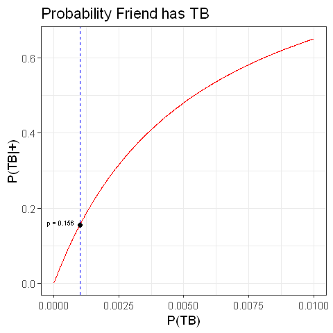
 we used to calculate our example above. Note that if the probability of contracting TB is 1%, then my friend would have nearly a 65% chance of having TB!(!!)
 . This is actually *never* true, because we do not have infinite sample sizes. The big joke in statistics is that, as a rule of thumb, once
  or so, then that’s large enough for the CLT to hold, and you can just apply tests that require it. Does no one see the madness behind this? Moreover, the CLT is not very robust to *highly skewed* data, which means that the “rule of thumb” actually doesn’t even work if you use a data set that is, I dunno, from any actual population? If your data is from leaf life people, or observations, chances are it will not be nice and normally distributed. Skew hurts every test, including the t-test, and if it’s bad enough, no amount of praying to the central limit theorem will fix that.]
 , where the function
  is observed in the observed case.”. Here
  refers to a statistical test, and
  , but not everyone finds this to be a useful substitution. Bayesians, of course, advocate for bayesian statistics instead, though that itself is not without its problems. As researchers, there is the more immediate problem of our employers and PI’s expecting p-values. Old habits die hard, and in order to get published, you have to reject the hell out of some hypotheses. It is not good enough to say “We thought maybe these two things are associated, but turns out they are not.
  “. While you won’t get published over such a claim, it is actually fallacious to think that the non-rejection of a null gives no information. Add in the fact that scientific research is based on “discovery”, and you have a recipe for accidental data dredging in order to achieve significant results.
 to a decision? I think maybe not, but causal modeling, probably yes.
 on the hold out set. “Machine learning is just a black box!” Maybe, but there is
  is measurable, and let
  be a sequence of non-negative, measurable functions such that, for
  ,
,
 be defined by
  as
as 
 implies that


 , for every intger
  , and the
  are bound below by 0, we have
 , for every
  . And so, taking the supremum for
  and passing to the limit gets
 .
.
 ,
,
 and
and  . Let
. Let  be, of course, the outer Lebesgue measure. Suppose that we have a set
  . In this case, it is possible to cover
  with a sequence
  of elementary sets, that is
  . Note that since
  is elementary, they may be written as a finite union of disjoint intervals
  ,
,  , for every integer
  , where
  are the end points of the interval
  .
. . Note that
  . Hence,
  , but the additivity of
  .
. . Now, it is possible to choose these elementary coverings of
  .
. .
. .
.

 as
as  was arbitrary.
 , where
  . Now, writing each
  which implies that
 ,
, , we can find a sequence of elementary sets so that
 ,
, can be obtained, which gives
 , for any
  such that
  , where
  is the outer Lebesgue measure.
 , which is known to be countable. So, the elements of the rational numbers may be enumerated so that
 . Now, fix
  and around each each
  , center an interval of length
  . That is, form the interval
 .
. forms an open set, which will be called
  . Now, the outer lebesgue measure is subadditive, so it follows that
 .
.